
Concepts - NLP, Multilabel Classification, Imbalanced Dataset, Text Embedding
The internet has become an integral part of modern society and has greatly impacted the way we communicate and access information. While it provides many benefits, it also has its downsides, one of which is the prevalence of toxic comments. In this project, I attempt to solve the problem we have with toxicity on the internet by building a machine learning model that detects these toxic comments.
Table of Contents
- Introduction
- Exploratory Data Analysis
- Data-mining with Regex
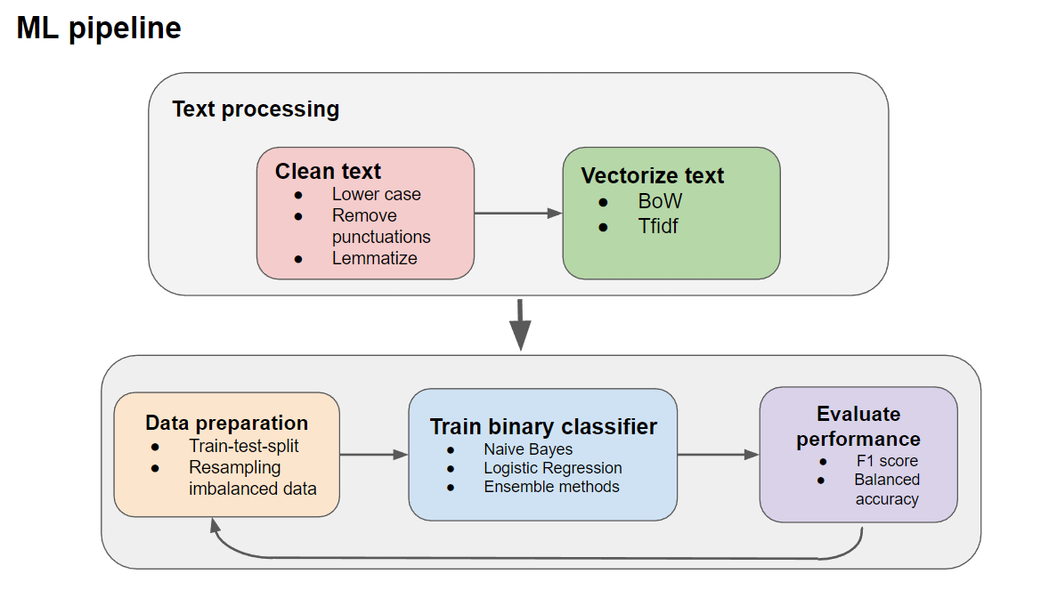
- Machine Learning Overview
- Text Cleaning
- Text Embedding
- Dealing with Imbalanced Dataset
Introduction: Why toxic comment filtering is important?
The internet has become an integral part of modern society and has greatly impacted the way we communicate and access information. While it provides many benefits, it also has its downsides, one of which is the prevalence of toxic comments. Toxic comments are comments that are harmful, offensive, or disruptive to a particular community or individual. They can take many forms, such as hate speech, personal attacks, and bullying.
It is important to filter out toxic comments on the internet because they can seriously impact individuals and communities. For example, toxic comments can lead to feelings of anxiety, depression, and low self-esteem, especially among young people who are still developing their sense of identity. This can cause long-lasting harm to their mental health and well-being. In some cases, toxic comments can even lead to self-harm or suicide. Moreover, toxic comments can also create an unhealthy and hostile environment for communities. They can drive away members, stifle creativity and innovation, and negatively impact the overall quality of a platform. This can lead to a decline in user engagement and satisfaction, which can have serious consequences for online businesses and websites. It is also important to consider the larger social implications of toxic comments. They can perpetuate harmful stereotypes, discrimination, and prejudice, and contribute to a divisive and toxic online culture. This can have a ripple effect on offline communities, leading to further social and political polarization.
Exploratory Data Analysis
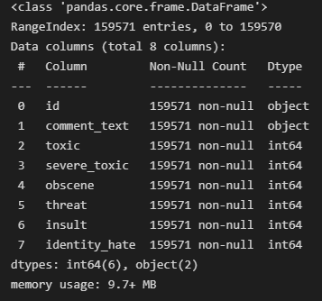
The dataset comes from Kaggle Toxic Comments Classification, a very popular dataset for NLP projects. The first thing to do is to explore the features and nuances of this dataset. The specific machine learning problem is a multilabel binary classification on text data. Summary points about this data:
- There are ~ 160 000 data points
- 6 distinct toxicity labels, not mutually exclusive
- Labels are encoded in 1s and 0s, binary classes
Taking a quick glance at the dataset with df.info() and df.head().
I want to know how often each label occurs in the dataset. It turns out that it is quite imbalanced.
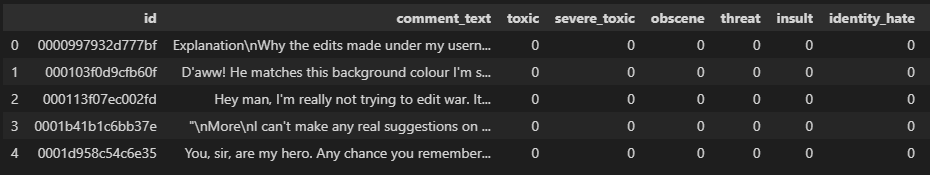
Print out of the first 5 rows of the dataset.
</n>
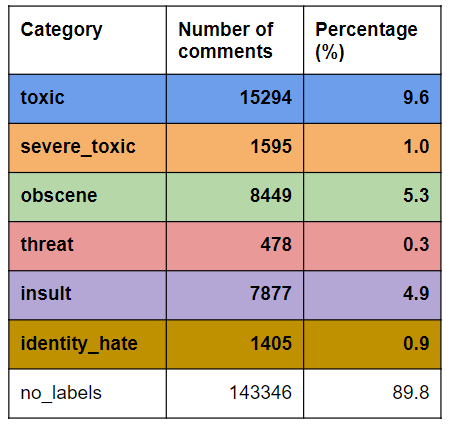
The proportion of comments that are labeled. About 89.8% of the comments are not toxic (no_labels). Therefore, the dataset is very imbalanced, which presents a challenge when training any ML model.
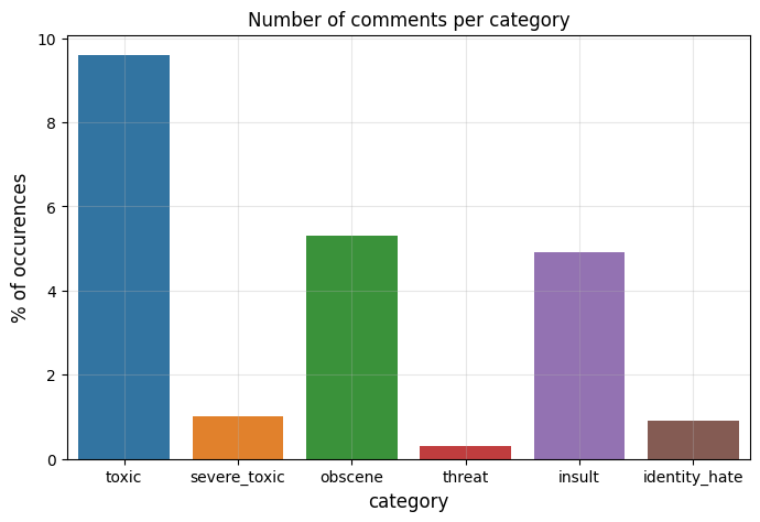
Bar graph representation of the table above. “Toxic” is the most common label at 9.6%. Severe_toxic, identity_hate, and threat occurs less than 1%, making them especially hard for the ML model to identify.
Since the labels are not mutually exclusive, some comments are often tagged with more than one of the toxicity categories. Below is bar graph depiction of the count of comments based on the total number of labels. Note there exist comments with all 6 labels; as you can imagine these comments are especially toxic 😅.
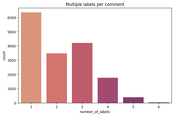
Distribution of comments with multiple labels.
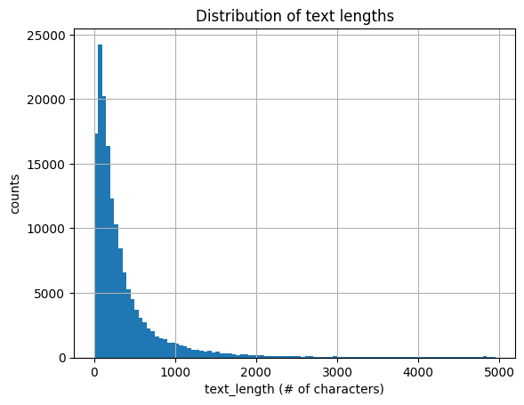
I calculated the text lengths for each comment because I wanted to know if it had a correlation with any of the toxicity labels. My hypothesis is that toxic labels would have longer comments. I first analyzed the distribution of text lengths. The average comment is 394.1 characters (67.3 words) and the longest comment is 5000 characters (1411 words). The fact that 5000 is such a conveniently round number seems that this was a cut-off set by the creators of the dataset.
Since comments can be tagged with more than one of the 6 labels, it is possible that the labels are somewhat correlated. Pearson correlation analysis between the labels is presented below; 1 being perfectly correlated, 0 having no correlation, and -1 being perfectly anti-correlated. It turns out that text length has very little correlation with the labels, which proves my hypothesis wrong.
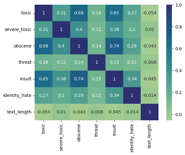
Pearson correlation heatmap of each toxicity label and text_length.
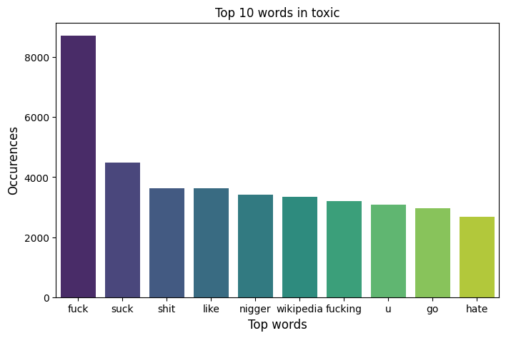
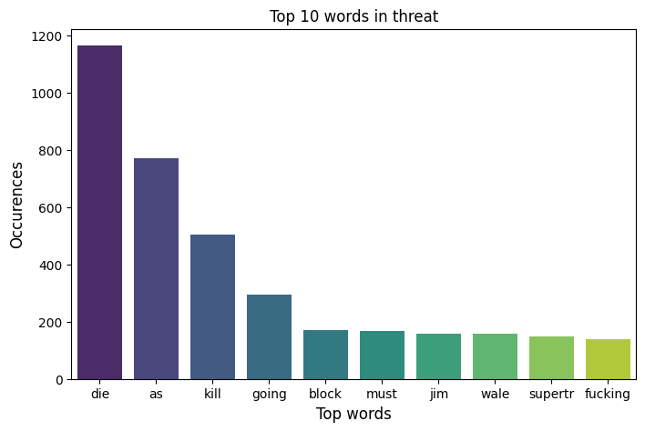
Word clouds are a fun way to visualize the frequency of words in a corpus of text. At first glance, it just seems like just a jumble of really profane words. But there is a noticeable difference between the different types of toxic labels. Here I posted the word cloud for all comments labeled “toxic” and “threat”. Notice the differences between the top 10 words in each subcategory.
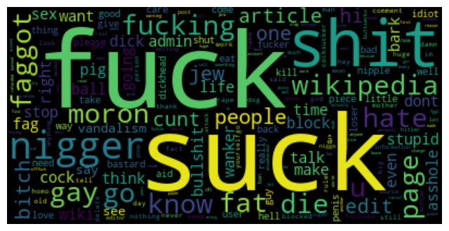
Word cloud for comments labeled “toxic”.
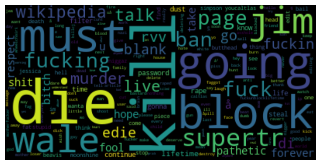
Word cloud for comments labeled “threat”.
Data-mining with Regex
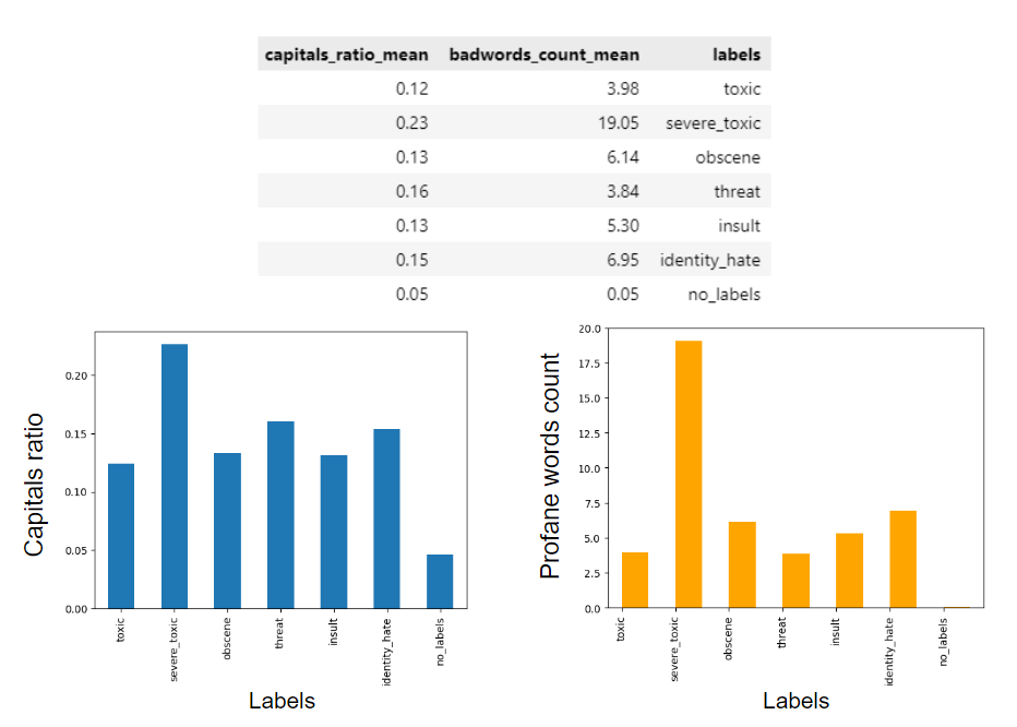
One thing I notice when randomly sampling the toxic comments is that some of them are written in all capitals or have excessive use of profane words. In order to analyze this, I used regex to extract information about the proportion of capital letters and profane words for each comment, and assign them to a new column in the dataframe. Here is a snippet of the regex code I used.
def find_capitals(text):
    matches = re.findall(r"[A-Z!]", text)
    return len(matches)/len(text)

df['capitals_ratio'] = df['comment_text'].apply(find_capitals)
With the newly created metrics, that is the capitals ratio and bad words count, I can aggregate these numbers and find the average for each label. The results are presented below in a table and respective bar graphs. This analysis shows that the use of capitals is significantly higher in toxic comments compared to clean comments, and likewise, for the profane words count. The more interesting finding is the noticeable differences between “severe toxic” compared to the rest of the labels, showing a higher proportion of capital letters and profane words. Given this finding, perhaps these two metrics can serve as additional training features to aid in the machine learning classification process.
Machine Learning Overview: Multilabel Classification problem
The input variables are the comments texts, and the response variables are the toxic labels. Since there are six labels that are not mutually exclusive, this is a multilabel binary classification problem. Furthermore, the dataset is very imbalanced, having the majority of comments being non-toxic (negative) and <10% being labeled (positive) any one of the toxic categories, with some labels occurring at < 1%.
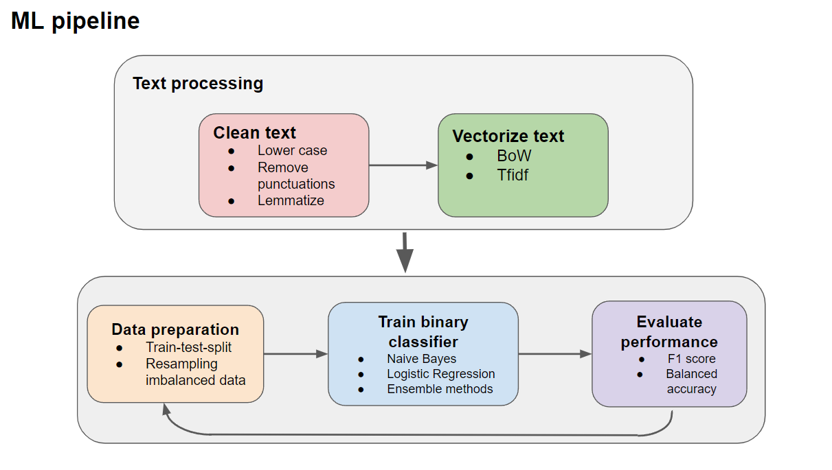
Text Cleaning
Standard text cleaning was performed on the raw comment text. I used NLTK library in Python, but it can be easily done with SpaCy library as well. Text cleaning process includes:
- lowercasing all letters
- stripping of extra whitespaces
- converting all contractions e.g. isn’t -> is not
- removing punctuations
- removing stopwords
- lemmatization of all words
I put all the text cleaning steps into a single function named text_cleaner(). Below is a printed sample of the text_cleaner output.
train_df['cleaner_text'] = train_df['comment_text'].map(lambda comments:   text_cleaner(comments))

seed=42
print(train_df['comment_text'].sample(random_state=seed).values)
["Geez, are you forgetful!  We've already discussed why Marx  was  not an anarchist, i.e. he wanted to use a State to mold his 'socialist man.'  Ergo, he is a statist - the opposite of an  anarchist.  I know a guy who says that, when he gets old and his teeth fall out, he'll quit eating meat.  Would you call him a vegetarian?"]

print(train_df['cleaner_text'].sample(random_state=seed).values)
['geez forgetful already discussed marx anarchist ie wanted use state mold ocialist man ergo statist opposite anarchist know guy say get old teeth fall quit eating meat would call vegetarian']
Although text cleaning makes the text unreadable based on conventional English grammar rules, it is easier for ML models to process.
Text Embedding
In order for the machine learning models to work on our text data, the raw text needs to be embedded into trainable data. The traditional way to do this is to vectorize each corpus of text. There are two common options from the sklearn library: CountVectorizer (bag-of-words) or TfidfVectorizer. Both vectorization processes removes context from the text and only considers the frequency of word occurence. The difference between them is that TFIDF gives more weight to words that don’t appear frequently in other documents (comments in this case), whereas bag-of-words doesn’t consider document frequency at all and treats each comment independently. In order to compare the performance of both vectorizers, I will apply both vectorizers and train with Logistic Regression classifier as a baseline model.
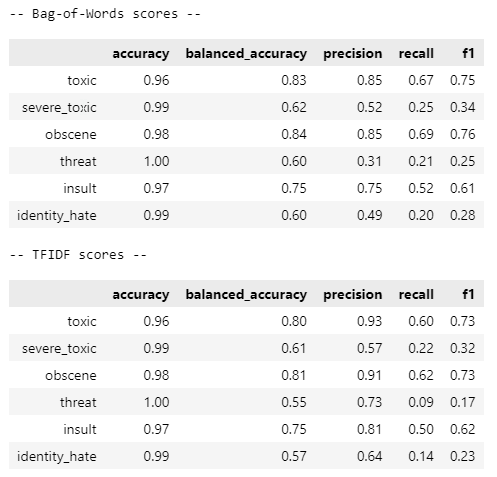
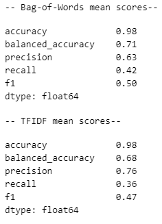
The accuracy score is quite high, which gives a misleading assessment of how well the ML model is performing because of the imbalanced nature of the dataset. For instance, accuracy is 100% for the threat label yet balanced accuracy and F1 score is extremely low. Balanced accuracy is a metric that accounts for false predictions, therefore is more suitable for assessing imbalanced data. Precision and recall scored really badly for both vectorizers, especially for rare labels (severe toxic, threat, identity hate). Assessing the performance of each vectorizer in the aggregate, bag-of-words performed slightly better, especially when looking at balanced accuracy and F1 score (the harmonic mean of precision and recall).
There is the question of which metric is the more important, precision or recall? Or both are equally important, therefore we should optimize for F1 score. Let’s first lay out some defintions
TP = True Positive, FP = False Positive, TN = True Negatives, FN = False Negatives
Precision = TP/(TP+FP)
Recall = TP/(TP+FN)
FP = good comments wrongfully labeled toxic
FN = undetected toxic comments
Precision is a measure of true positives (correctly labeled toxic comments) relative to false positives (clean comments wrongfully labeled toxic). Recall measures true positives relative to false negatives (toxic comments that were not detected). It really depends on your specific application of the toxic comments filtering. For example, if there are a lot of kids in the platform, then high recall is preferred at the expense of some wrongfully filtering good comments. If the platform is intended for more candor and certain adult style humor, then high precision is preferred. Since I cannot decide between the two, I will optimize for F1 score for the rest of this project.
For a really good explanation of all these metrics I discussed, read this blog: https://neptune.ai/blog/balanced-accuracy
Dealing with an imbalanced dataset
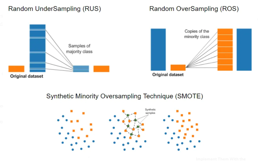
A major reason why the models show such poor performance for rare labels is because of the imbalanced dataset. There are a few techniques we can try to deal with this imbalance, which involve selectively sampling the training data to create balance. Here are the techniques:
Random Under-Sampling (RUS): Randomly sample from the majority class and leave the minority class alone.
Random Over-Sampling (ROS): Randomly sample from the minority class with replacement, therefore some data points will be sampled repeatedly, and leave the majority class.
Synthetic Minority Over-Sampling Technique (SMOTE): Same concept as ROS, but rather than repeatedly sampling the same few data points, data is synthetically created by interpolation. This is to mitigate the overfitting problem present in ROS, however, requires more computing power.
In the next ML pipeline, I will use RUS and SMOTE resampling of the training data, and compare it with the original dataset. The classifier I used is Logistic Regression since it has been a baseline model. The dataset is first resampled with RUS, SMOTE or left alone, then split 75%/25% for training and validation. The performance metrics I chose were balanced accuracy, precision, recall, and F1, and these were evaluated using the validation dataset. I decided to plot the scores for each label class separately to visualize the variance between them, since their respective imbalances play a signficant role in the evaluation scores.
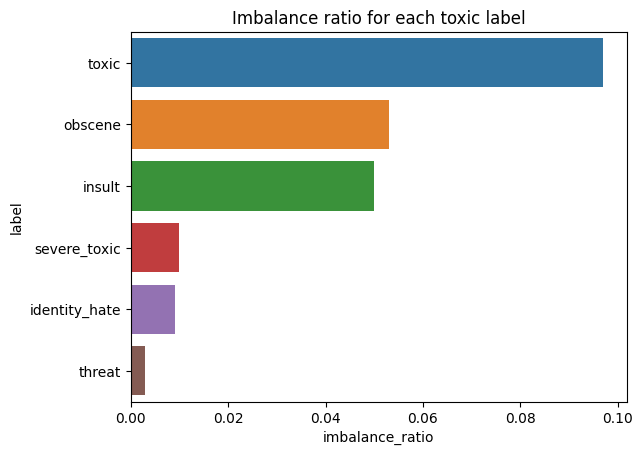
Imbalance ratio is just the proportion of each label present in the entire dataset.
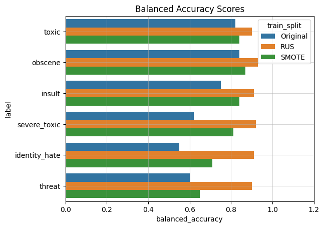
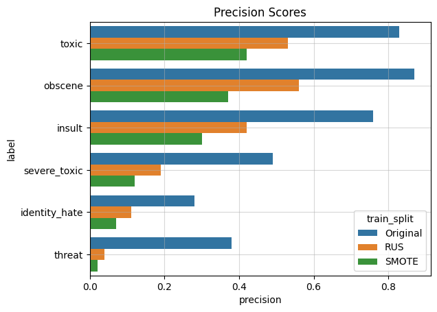
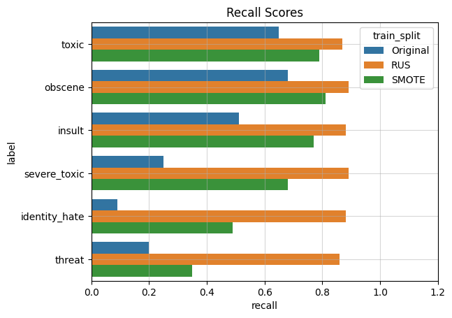
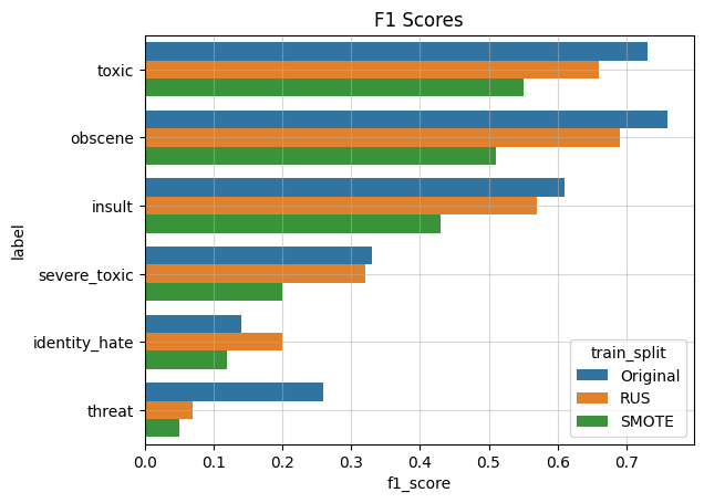
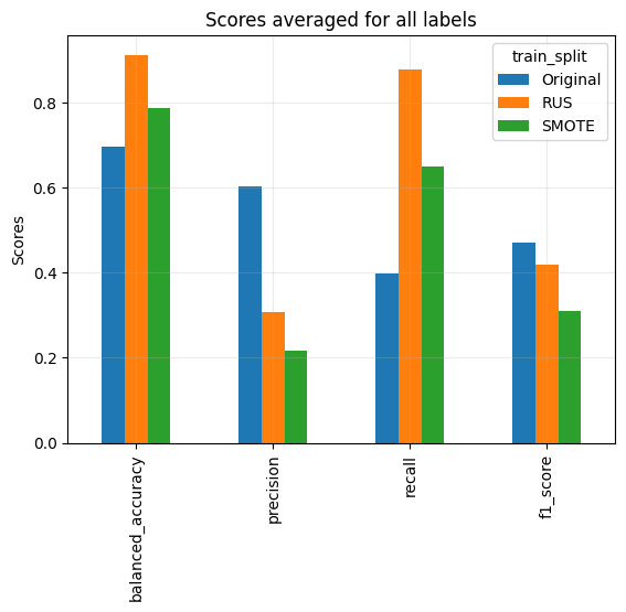
It turns out that resampling the dataset improves certain metrics but compromises others. Both RUS and SMOTE improves balanced accuracy and recall, yet sacrifice precision. Overall RUS performs better than SMOTE.