

The Toxic Comments Kaggle dataset is widely recognized as a valuable resource and serves as a prominent benchmark for multilabel text classification. I invite you to take a look at my insightful blog post where I delve into the exploration of this dataset and apply simple machine learning algorithms with resampling methods for treating imbalanced datasets. Within this work, I utilize cutting-edge deep learning models implemented with the Tensorflow and Pytorch frameworks. Moreover, I conduct a comprehensive comparison of various methodologies to effectively tackle the task of multi-label text classification.
Importing and cleaning data set
The text cleaning function can be found in my previous work on the toxic comments dataset. I’m conveniently import those functions to streamline the text preprocessing. Then I use scikit-learn CountVectorizer to the the basic embeddings. I chose CountVectorizer as a baseline text embedding for it’s simplicity and ease of interpretation. However, there are definitely more advanced text embeddings that may perform better for this specific case of multi-label text classification.
# importing dataset from local directory
dataset_directory = ".../toxic-comments-datasets/"
train_df = pd.read_csv(dataset_directory + "train.csv.zip", usecols = ['comment_text', 'toxic', 'severe_toxic', 'obscene', 'threat', 'insult', 'identity_hate'])
train_df = train_df.astype({'toxic':'int16',
                            'severe_toxic':'int16',
                            'obscene':'int16',
                            'threat':'int16',
                            'insult':'int16',
                            'identity_hate':'int16'})

train_df = train_df.dropna()  # I found 5 nan rows in cleaned_text, so I just drop those rows altogether

# importing custom text_cleaner
from text_cleaning_functions import text_cleaner
train_df['cleaner_text'] = train_df['comment_text'].map(lambda comments : text_cleaner(comments))
# create text embeddings with scikit-learn CountVectorizer
LABELS = ['toxic', 'severe_toxic', 'obscene', 'threat', 'insult', 'identity_hate']
train_text = train_df['cleaner_text']
train_labels = train_df[LABELS]

train_text_countvec = CountVectorizer(max_features=10000).fit_transform(train_text)

X_train, X_test, y_train, y_test = train_test_split(train_text_countvec, train_labels.values, test_size=0.2)
print(X_train.shape)
print(X_test.shape)
TensorFlow MLP model
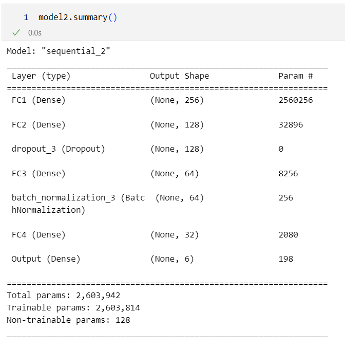
The architecture I’m using is a very general Multilayer Perceptron (MLP), with multiple fully connected layers, a single dropout layer, and batch normalization layer. The topology of this architecture tapers from a large input of N-vector embeddings of the text to be classified, towards the 6 binary classes of the multi-label classification problem.
import tensorflow as tf
from tensorflow.keras import layers

l2_regularizer = tf.keras.regularizers.L2(l2=0.001) # default l2 =
glorot_initializer = tf.keras.initializers.GlorotNormal(seed=32)

model2 = tf.keras.Sequential([
    layers.Input(shape=X_train.shape[1:], name="Input_Layer"),

    layers.Dense(256,
                 activation="relu",
                 kernel_initializer=glorot_initializer,
                 kernel_regularizer=l2_regularizer,
                 bias_regularizer=l2_regularizer,
                 name="FC1"),

    layers.Dense(128,
                 activation="relu",
                 kernel_initializer=glorot_initializer,
                 kernel_regularizer=l2_regularizer,
                 bias_regularizer=l2_regularizer,
                 name="FC2"),

    layers.Dropout(rate=0.3),

    layers.Dense(64,
                 activation="relu",
                 kernel_initializer=glorot_initializer,
                 kernel_regularizer=l2_regularizer,
                 bias_regularizer=l2_regularizer,
                 name="FC3"),

    layers.BatchNormalization(),

    layers.Dense(32,
                 activation="relu",
                 kernel_initializer=glorot_initializer,
                 kernel_regularizer=l2_regularizer,
                 bias_regularizer=l2_regularizer,
                 name="FC4"),

    layers.Dense(y_train.shape[1],
                 activation="sigmoid",
                 kernel_initializer=tf.keras.initializers.GlorotNormal(seed=3),
                 kernel_regularizer=l2_regularizer,
                 bias_regularizer=l2_regularizer, name="Output")
])
#compile
model2.compile(optimizer=tf.keras.optimizers.Adam(learning_rate=0.001),
              loss='binary_crossentropy',
              metrics=["binary_accuracy"])
Hyperparameters explained:
kernel_initializer is a parameter used in neural networks to define the method for initializing the weights (also called “kernels”) of the layers. Proper weight initialization is crucial for training a neural network because it can affect the speed of convergence and the final performance of the model.
There are several weight initialization techniques available, and some of the most common ones include:
-
Random initialization: Randomly initializing the weights with small values, usually sampled from a uniform or normal distribution.
-
Xavier/Glorot initialization: Initializing the weights by drawing samples from a uniform distribution with a specific range. This range depends on the number of input and output units in the layer. The idea behind Xavier initialization is to maintain a similar variance for both input and output activations during the forward pass, which helps with training deep networks.
-
He initialization: Similar to Xavier initialization, but it uses a different range for the uniform distribution, making it more suitable for networks using ReLU (rectified linear unit) activation functions.
kernel_regularizer is a parameter used in neural networks to apply regularization on the weights (also called “kernels”) of the layers. Regularization is a technique used to prevent overfitting by adding a penalty term to the loss function, which discourages the model from learning overly complex or noisy patterns in the training data. The primary goal of regularization is to improve the model’s generalization ability, so it performs well on unseen data.
There are two main types of regularization applied to weights:
-
L1 regularization (Lasso): Adds the absolute values of the weights to the loss function, scaled by a regularization factor (usually denoted by lambda or alpha). This type of regularization encourages sparsity in the model, as some weights may be driven to zero.
-
L2 regularization (Ridge): Adds the squared values of the weights to the loss function, scaled by a regularization factor. L2 regularization discourages large weight values but doesn’t necessarily drive them to zero. It’s commonly used in neural networks.
Training the compiled NN model
# this step is necessary to convert the sparse matrix to a sparse tensor

def convert_sparse_matrix_to_sparse_tensor(X):
    coo = X.tocoo()
    indices = np.mat([coo.row, coo.col]).transpose()
    return tf.SparseTensor(indices, coo.data, coo.shape)

train_tensor = convert_sparse_matrix_to_sparse_tensor(X_train)
train_tensor = tf.sparse.reorder(train_tensor)
test_tensor = convert_sparse_matrix_to_sparse_tensor(X_test)
test_tensor= tf.sparse.reorder(test_tensor)

# train for 10 epochs
history = model2.fit(train_tensor, y_train,
                     validation_data=(test_tensor, y_test),
                     epochs=10)

Pytorch MLP model
For the sake of comparison and learning, I created an equivalent neural network with PyTorch.
import torch
import torch.nn as nn
import torch.nn.functional as F
import torch.optim as optim
from torch.nn import init

class CustomModel(nn.Module):
    def __init__(self, input_shape, output_shape):
        super(CustomModel, self).__init__()

        self.fc1 = nn.Linear(input_shape, 256)
        self.fc2 = nn.Linear(256, 128)
        self.fc3 = nn.Linear(128, 64)
        self.bn = nn.BatchNorm1d(64)
        self.fc4 = nn.Linear(64, 32)
        self.fc5 = nn.Linear(32, output_shape)

        self.dropout = nn.Dropout(p=0.3)

        self.init_weights()

    def forward(self, x):
        x = F.relu(self.fc1(x))
        x = F.relu(self.fc2(x))
        x = self.dropout(x)
        x = F.relu(self.fc3(x))
        x = self.bn(x)
        x = F.relu(self.fc4(x))
        x = torch.sigmoid(self.fc5(x))
        return x

    def init_weights(self):
        for m in self.modules():
            if isinstance(m, nn.Linear):
                init.xavier_normal_(m.weight, gain=1)
                init.constant_(m.bias, 0)

                # Apply L2 regularization to weights and biases
                # Note that the equivalent is handled in the optimizer in PyTorch
                # See the optimizer definition below

input_shape = X_train.shape[1]
output_shape = y_train.shape[1]

model = CustomModel(input_shape, output_shape)

# Define an optimizer with L2 regularization (weight_decay)
optimizer = optim.Adam(model.parameters(), lr=0.001, weight_decay=0.001)
criterion = nn.BCELoss() # Use Binary Cross Entropy Loss for binary classification
# convert the training and test data to usable torch tensors
X_train_dense = X_train.toarray()
X_test_dense = X_test.toarray()

X_train_tensor = torch.tensor(X_train_dense, dtype=torch.float32)
y_train_tensor = torch.tensor(y_train, dtype=torch.float32)
X_test_tensor = torch.tensor(X_test_dense, dtype=torch.float32)
y_test_tensor = torch.tensor(y_test, dtype=torch.float32)
from torch.utils.data import TensorDataset, DataLoader

batch_size = 64

train_dataset = TensorDataset(X_train_tensor, y_train_tensor)
train_loader = DataLoader(train_dataset, batch_size=batch_size, shuffle=True)

test_dataset = TensorDataset(X_test_tensor, y_test_tensor)
test_loader = DataLoader(test_dataset, batch_size=batch_size, shuffle=False)
Setting the training loop
epochs = 10

for epoch in range(epochs):
    model.train() # Set the model to training mode

    # Training loop
    for i, (inputs, targets) in enumerate(train_loader):
        optimizer.zero_grad() # Reset the gradients
        outputs = model(inputs) # Forward pass
        loss = criterion(outputs, targets) # Compute the loss
        loss.backward() # Backward pass
        optimizer.step() # Update the weights

    # Validation loop
    model.eval() # Set the model to evaluation mode
    validation_loss = 0
    for inputs, targets in test_loader:
        with torch.no_grad():
            outputs = model(inputs) # Forward pass
            loss = criterion(outputs, targets) # Compute the loss
            validation_loss += loss.item()

    validation_loss /= len(test_loader)
    print(f"Epoch {epoch+1}/{epochs}, Validation Loss: {validation_loss:.4f}")
Conclusion
Differences between Tensorflow and Pytorch
The first difference is the API and code syntax for implementing both packages. The typical workflow for implementing deep learning models:
- create model → compile → fit/train → predict.
- I find that the Tensorflow API a bit more intuitive, however, I’m sure it’s a matter of taste.
- Pytorch was significantly faster at training compared to Tensorflow.
- There’s more code in Pytorch to implement the same NN model.
The accuracy and loss of both models were very close, which is no surprised because the NN architectures were the same. The difference is primarily in implementation and speed of processing.
What’s next?
- Implement different text embeddings e.g. BERT, GloVe
- Experiment with different NN architectures