

Concepts - Monte-Carlo simulation, price modeling, statistical modeling
I built a Monte-Carlo simulation based on the Poisson process to model the price dynamics of a ride-hailing business. Simulations provided projections of earnings and profit of the company for a 1-12 month period. Strategies for improving profitability are written at the end of this report.
Original report is written here
–This post is still in draft phase until I figure out how to post latex equations in markdown–
Case Study
You’re launching a ride-hailing service that matches riders with drivers for trips between the Toledo Airport and Downtown Toledo. It’ll be active for only 12 months. You’ve been forced to charge riders $30 for each ride. You can pay drivers what you choose for each individual ride.
The supply pool (“drivers”) is very deep. When a ride is requested, a very large pool of drivers see a notification informing them of the request. They can choose whether or not to accept it. Based on a similar ride-hailing service in the same market, you have some data on which ride requests were accepted and which were not. (The PAY column is what drivers were offered and the ACCEPTED column reflects whether any driver accepted the ride request.)
The demand pool (“riders”) can be acquired at a cost of $30 per rider at any time during the 12 months. There are 10,000 riders in Toledo, but you can’t acquire more than 1,000 in a given month. You start with 0 riders. “Acquisition” means that the rider has downloaded the app and may request rides. Requested rides may or may not be accepted by a driver. In the first month that riders are active, they request rides based on a Poisson distribution where lambda = 1. For each subsequent month, riders request rides based on a Poisson distribution where lambda is the number of rides that they found a _match _for in the previous month. (As an example, a rider that requests 3 rides in month 1 and finds 2 matches has a lambda of 2 going into month 2.) If a rider finds no matches in a month (which may happen either because they request no rides in the first place based on the Poisson distribution or because they request rides and find no matches), they leave the service and never return.
Analyzing Driver Acceptance Data
My first task is to analyze the given driver acceptance data. There are 1000 ride requests, the PAY column is the pay offered to drivers, and the ACCEPTED column shows whether or not they accepted the ride offer. I plotted a stacked histogram (figure 1) to visualize the distribution of both accepted and not accepted rides as a function of pay offered to drivers. Regardless of acceptance, the distribution of all 1000 ride requests in the given data resembles a normal distribution centered around ~$28.

Modeling driver acceptance rate
Upon closer inspection of the data and distribution, I noticed that low pay has fewer accepted rides and high pay has more. To explore this further, I binned the data into pay ranges of $2 intervals and calculated the acceptance rate in each pay range bin and other useful metrics. You can see the newly binned data here.
I then fit the sigmoid model to the acceptance rate as a function of the pay range. The formula to model the acceptance rate is expressed as
Where
is the acceptance rate, which is simply
in each pay range,
is the pay range in $2 intervals,
is the width, and
is the offset. Here
and
are free parameters for fitting the model. Using standard curve fitting methods via scipy.optimize.curve_fit, we find that
and
.
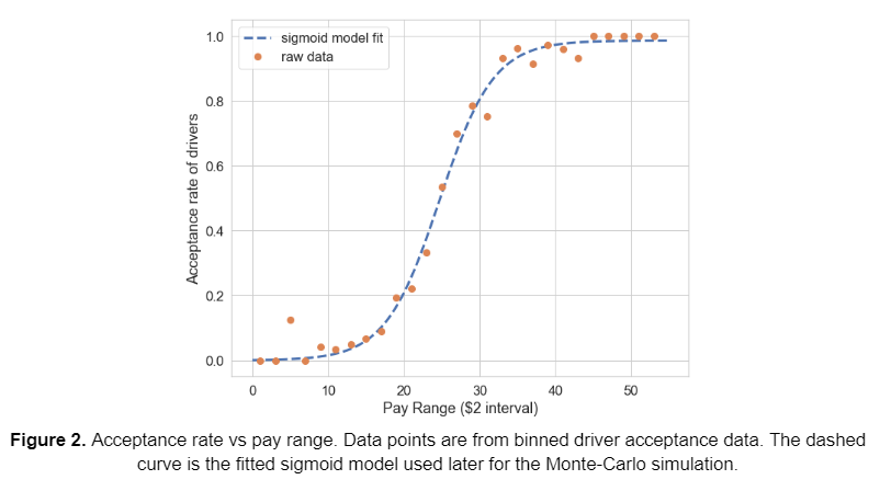
We can now use the above model as a function that outputs the average acceptance rate. This model will be used later in this report to model acceptance rates of drivers based on driver compensation.
Profit per ride request
A very relevant question to ask is: _what is the optimal driver compensation that maximizes total profit? _There is an inherent tradeoff between profit per ride and the acceptance rate of drivers. The company makes more profit per ride if we lower the driver compensation but less acceptance of rides from drivers, yielding fewer rides in total. To answer this question, we calculate profit per ride request in every pay range, essentially:
Where
represents the i-th pay range in our binned data. The results are plotted below. From our calculation, we see that the optimal pay range is $24-26, yielding about $2.69 profit per ride request.
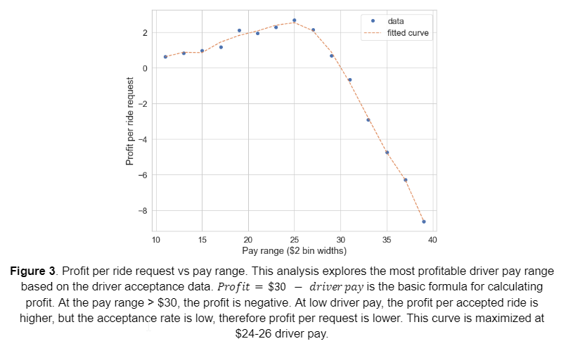
is the basic formula for calculating profit. At the pay range > $30, the profit is negative. At low driver pay, the profit per accepted ride is higher, but the acceptance rate is low, therefore profit per request is lower. This curve is maximized at $24-26 driver pay.
Caveat and assumptions
In the analysis presented above, we assume that the driver pool is not a limiting constraint, i.e., there are sufficient drivers to accept the ride offers. This assumption makes sense if the number of available drivers far exceeds the number of ride requests in a given day, or each driver can take multiple ride requests to fulfill all the rides requested.
In this case study, the rider pay is fixed at $30 per ride. Then the profit per ride is simply the rider fare minus the driver compensation. So if a driver’s compensation is $25, the company profits $30 - $25 = $5. This constraint for rider pay makes the case study easier to analyze, but perhaps having a flexible rider fare adjusted to the constantly fluctuating market supply and demand can generate more profit. For example, Uber adjusts their fares and compensation based on the time of day.
The model for driver acceptance rate is only based on driver compensation, which is the only data provided for this case study. However, one can imagine the decision of a driver accepting a ride is not solely based on compensation. A myriad of other factors should be considered. Just to list a few: time of day, day of the week, how many rides have the driver done, details about driver profile, etc. If it is possible for the app or software to record more data, then we can have more input into our model. A sigmoid equation was quite obvious with the given data in this case study. If the number of features gets too large, then perhaps machine learning models (specifically logistic regression supervised learning) are preferred over modeling with equations.
Modeling the number of rides with poisson statistics
Building the Monte-Carlo simulation
The next task is to model the month-to-month rider churn and ride requests given the description of rider behavior in the case study. Given the scenario described in this case study, I thought it would be most appropriate to model this with Monte-Carlo simulation.
- In the first month, riders who just download the app will request rides with a Poisson probability distribution of
.
- The number of ride matches shall be the: M = (number of requests) x (acceptance rate).
-
The acceptance rate (AR) is determined by driver compensation according to the fitted model described in the previous section. [1]
- In the subsequent month, each rider will request rides will follow
, where M is the number of matched rides from the previous month.
- Following these steps, one can simulate the month-to-month ride matches with random number generators that follow the Poisson distribution. In this work, I use scipy.stats.poisson.rvs to simulate the poisson statistics.
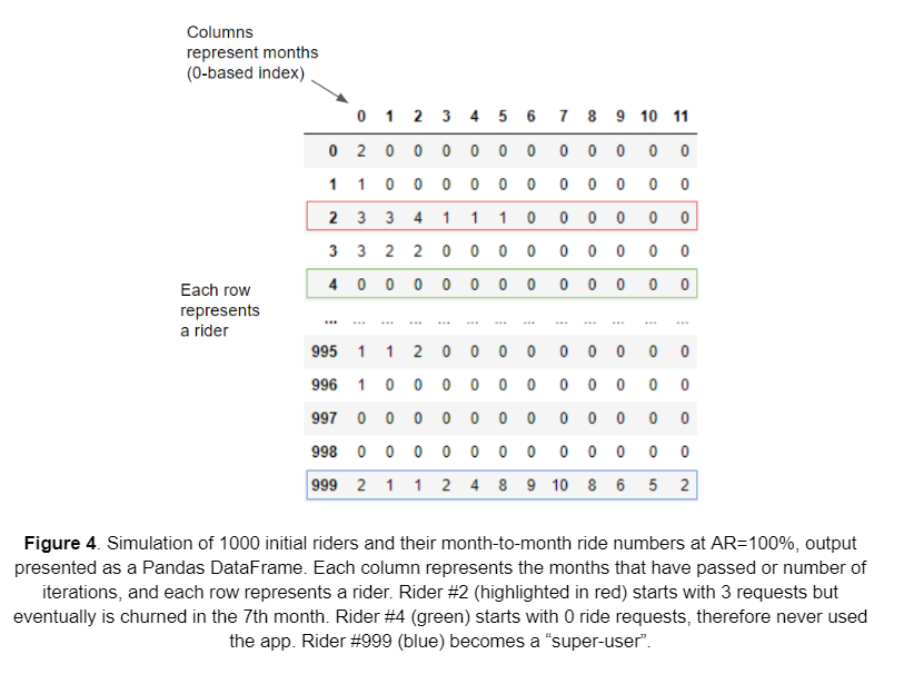
First we simulate the 1000 initial riders, with 100% AR every month, and initial distribution of
. The result of the simulation is presented in the pandas DataFrame below (only sampling the first and last 5 rows). The columns represent the months of simulation, the rows represent the n-th rider - note that python by default creates columns and rows with 0-based index. To interpret this simulation, rider #2 (red outline) has 3 rides the first month, 3 rides the second month, but in the 7th month completely stops using the app and has 0 rides. Some riders randomly start with 0 rides in the first month (rider #4 in green), while some riders become “super-users” and end up requesting rides a lot in the subsequent months (rider #999, outlined in blue)
Exploring the effect of acceptance rate (AR)
To visualize the distribution of rides in this simulation, I grouped the data by rides each month and plotted them in bar charts. I did this for 100% and 50% AR to see the effect it has on the number of rides month-to-month.
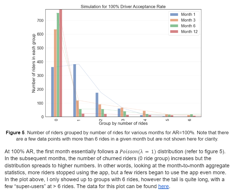
At 100% AR, the first month essentially follows a
distribution (refer to figure 5). In the subsequent months, the number of churned riders (0 ride group) increases but the distribution spreads to higher numbers. In other words, looking at the month-to-month aggregate statistics, more riders stopped using the app, but a few riders began to use the app even more. In the plot above, I only showed up to groups with 6 rides, however the tail is quite long, with a few “super-users” at > 6 rides. The data for this plot can be found here.
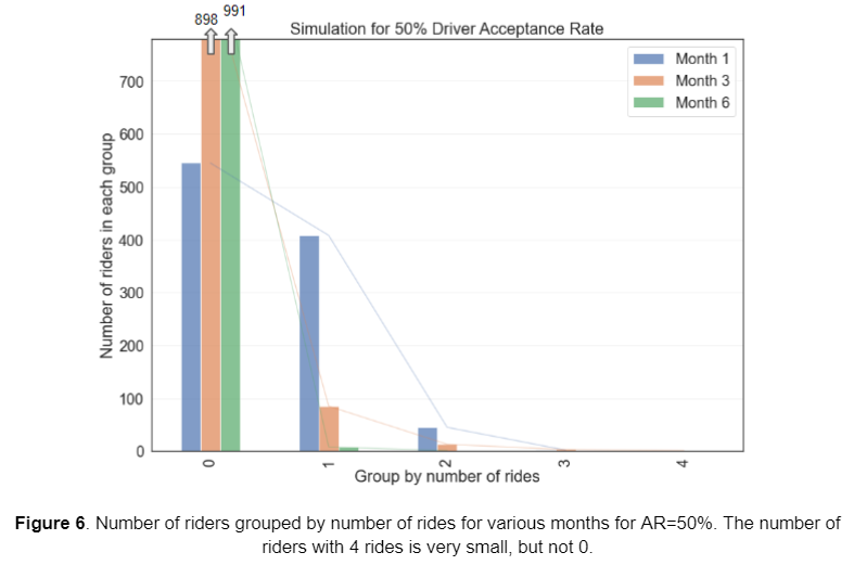
At 50% AR, the distribution becomes more narrow, and customer churn happens faster, which is no surprise (see figure 6, data can be found here). By the 3rd month, 898 out of 1000 (nearly 90%) initial users stopped using the app, and 991 out of 1000 (99%) stopped using it by the 6th month. Furthermore, almost no super-users (users with >4 rides in a given month) exist at 50% AR. The interpretation could be that if half the ride request doesn’t get matched, then a rider who actually needs a ride to/from the airport finds it too inconvenient to use the app, and eventually quits. This analysis illustrates the effect of the acceptance rate in the Monte-Carlo simulation and stresses the importance of having a high acceptance rate amongst drivers.
Total rides vs driver Acceptance Rates (AR)
A distinct problem of using random number generators to simulate the ride statistics is that the random number generator outputs a slightly different result every simulation run. Figure 7 shows an example of 5 different simulation runs using the same code. The entries in the table are the total rides of each month (columns) for different simulation runs (rows). The results are close with a relatively small variance, but never exactly the same.
– error –
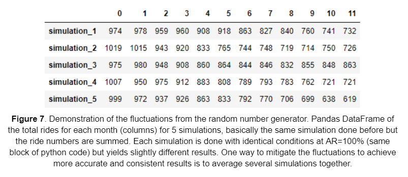
Next, I analyze the effects of AR on the total rides at each month and the total rides at the end of 12 months. In order to mitigate the fluctuations of the random number generator, I averaged the 10 simulation runs, each of 1000 initial riders.
Calculating month-to-month earnings[2]
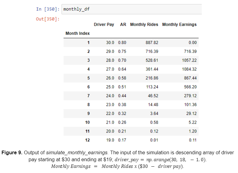
Next we build a model that calculates the earnings of the company per month based on the Monte-Carlo simulation I just built. Here we want the input to be driver pay (i.e. driver compensation) and infer the acceptance rate based on the sigmoid model detailed above (see figure 2). I wrote a function, simulate_monthly_earnings(), that takes an array of driver pays, each element in the array being the driver pay for that month, and outputs the month-to-month total rides and total earnings. It is worth mentioning again that high driver compensation yields higher AR but lower earnings per ride, and vice-versa. This dynamic trade-off makes for an interesting optimization problem.
– error –
– error –
.
– error –
.
Output of simulate_monthly_earnings function. The input is an array of driver pay for each month. AR is dependent on the driver’s pay according to the predefined sigmoid model. For each month the monthly rides and monthly earnings are calculated. Note that the earning is $0 for $30 driver pay because rider pay is equal to $30, which breaks even. The exact equation for earnings is
– error –
. Monthly Rides is determined by the Monte-Carlo simulation detailed in the previous section, but averaged over 100 simulations. The next step is to maximize total earnings summed over n_months.
Maximizing total earnings
For a systematic approach to maximizing the earnings, I came up with two general strategies:
- Keep the driver pay fixed across all months and find the driver pay value that maximizes the earnings for n months.
- Allow driver pay to be flexible month to month. This is harder to optimize computationally compared to the first strategy since we would have to find the argmax of many parameters (e.g. 12 choices for driver pay if simulated for 12 months), as opposed to one parameter in strategy #1.
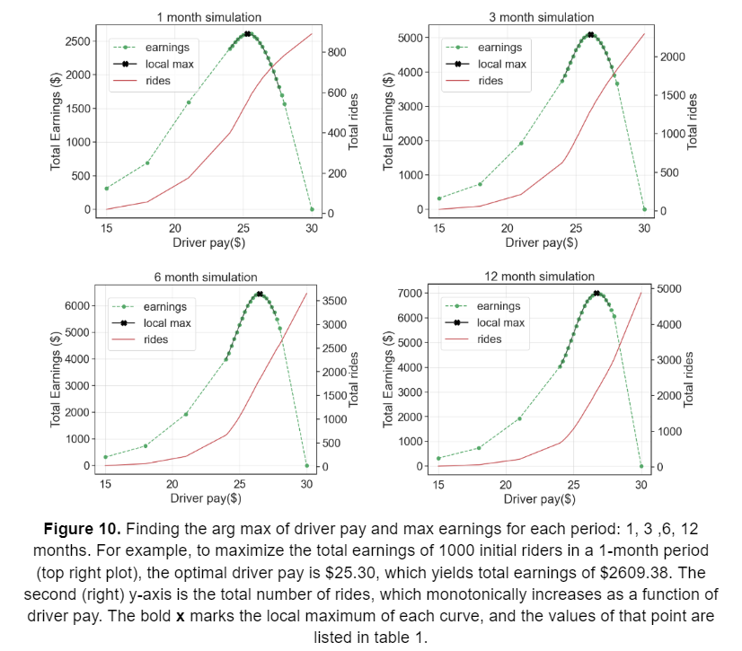
Using strategy #1 with fixed driver pay, I find the maximum earnings and argmax driver pay for 1-month, 6-month, and 12-month periods. The results are plotted below in figure 10. In this report, I will not present strategy #2 since it is a 12-parameter optimization problem and my computer was not able to solve it within a reasonable time. I tried strategy #2 by manually choosing the driver pay for every month and was able to get slightly better results than strategy #1, but was not worth the effort of doing it every time.
– error –
| Months | Optimal Driver Pay ($) | Maximized Total Earnings ($) |
| 1 | 25.3 | 2609.38 |
| 3 | 26.1 | 5092.82 |
| 6 | 26.6 | 6446.37 |
| 12 | 26.8 | 7009.55 |
Table 1. summary of the maximum points in figure 10.
The results of the simulation show a very interesting trend for the optimal driver pay depending on the number of months we are optimizing for. The simulation shows that lower driver pay is optimal for maximizing short-term earnings and vice-versa for maximizing long-term earnings. This can be explained by considering the trade-off between earnings per ride and reducing customer churn. Higher driver pay will have a higher driver acceptance rate, so therefore a higher number of rides, which in the long run, is better for total earnings. Therefore, earning less per ride but having more total rides may be better depending on which month we want to maximize earnings for. However, the number of rides and consequently the total earnings taper off quickly after a few months, which is noticeable in the relatively small difference in total earnings between the 6-month and 12-month simulations.
Summary of results
Why is it not profitable?
Assuming the Monte-Carlo simulation I built accurately models the rider and driver behaviors described in the case study, then I have effectively proven that it is impossible for the company to make a profit. All the simulations presented above were for 1000 initial riders, which is a $30,000 initial acquisition cost. The simulations show that the most the company can earn after 12 months is ~$7000, which is a net loss of about ~$23,000. There are a few reasons why the scenario in this case study cannot be profitable:
- The Poisson process that models rider requests has a very high month-to-month churn rate, even with AR=100%. This is because the distribution of ride requests starts at
– error –
and 37% is churned in the next month (i.e.
– error –
). When this process is simulated for 12 months at 100% AR, only ~15% of the initial number of riders remain using the app.
- The profit margin per ride is too low. Either the rider pay of $30 is not enough, or the driver pay is too high for a given acceptance rate.
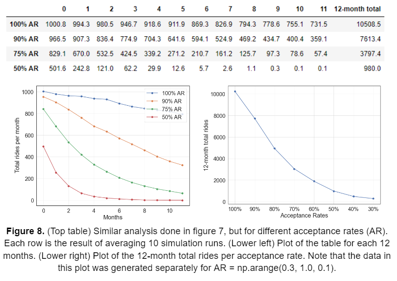
- The driver acceptance rate makes a huge difference in this model. Figure 8 depicts the effect acceptance rate on the total ride statistics. At the end of 12 months, simulation for AR=100% has ~10000 total rides, while AR=50% has ~1000 total rides, a factor of 10 decreases as a result of ½ the acceptance rate.
How to become profitable?
Given that scenario in the case study is not profitable, let’s explore the conditions that allow positive profits outside the constraints of the case study.
Increasing rider pay is one of the most straightforward ways to increase earnings. Take the 12-month situation in the analysis presented in figure 8, where the maximum earnings are ~$7000 at $26.80 driver pay, 62.8% AR, and 2188 total rides.With the rider acquisition cost of $30000 for 1000 initial riders, the net loss is then -$23,000. The required extra earnings per ride to reach break even is $23,000/2188 = $10.5, which means that each ride should cost the rider $30 + $10.5 = $40.5. The caveat is that this calculation is only valid if the extra cost does not affect the rider’s behavior, which is an unlikely assumption for such a steep increase in the rider fare. However, increasing the rider fare by some amount seems to be an effective approach, but the exact amount will depend on how it affects supply and demand dynamics.
Another approach is to reduce total customer churn or reduce the month-to-month churn rate. The churn is affected by two parameters, the acceptance rate and the previous ride number i.e.
– error –
parameter in the Poisson distribution. Starting the process with
– error –
at 100% AR, about 36.8% of riders are churned in the first month then 85% of customers are churned by the end of 12 months. Considering the high cost of initial rider acquisition ($30 per rider), it seems like a huge waste to have most of these riders completely stop using the app. Therefore, it would be very beneficial to keep the existing riders from quitting the app. Perhaps a more targeted rider acquisition approach, where only the very interested users are given the app in the beginning.
_What if the AR is higher for lower driver pay? _In the case of 100% AR, the initial 1000 riders in the system will accumulate ~10500 rides in 12 months (see figure 8). If the earnings per ride are just $3 (driver pay = $27), then there will be profitable by the end of 12 months. However, at $27, the AR is actually ~65% based on the given driver acceptance data (see figure 2), which yields approximately ~2500 total rides by the end of 12 months. If it is at all possible to improve the acceptance rate for lower driver pay, then the sweet spot is around 100% AR at $27.
In conclusion, even though profitability is not feasible in the original scenario, the work and analysis presented above elucidated an approach to maximizing revenue given a target period (n_months). My analysis coupled with the Monte-Carlo simulation also revealed the long-term behaviors of the riders and drivers, as well as churn rate dynamics as a function of driver compensation, which can be invaluable information that aids company executives in making policy decisions that will improve long-term profits. Note that the analysis I presented primarily focused on the 12 month period or shorter, but my Python code can be generalized for any period of time and any changes in the pricing parameters.
Notes
[1] In the following sections, I will simulate the month-to-month number of rides, which is essentially the number of ride matches. This is not to be confused with ride requests. In the case of 100% AR, ride request is equal to number of rides.
[2] Note that I intentionally used the term “earnings” instead of “profit” to refer to the amount of money the company takes home for each ride. Earnings = rider_pay - driver_pay. I define “Profit” as the difference between earnings and rider acquisition cost.